AI & Machine Learning
Clustering Algorithms: How to Choose the Right One
Compare clustering algorithms like k-means, HDBSCAN and DTW, avoid the pitfalls, and prove your clusters are real. Read the practical guide now.
Rodrigo Acosta
21 min read
Compare clustering algorithms like k-means, HDBSCAN and DTW, avoid the pitfalls, and prove your clusters are real. Read the practical guide now.
Rodrigo Acosta
A team runs k-means on a customer table, gets five tidy colored blobs on a scatter plot, and ships "five segments" to the business. Nobody asks the awkward question: would the same pipeline have produced five equally tidy blobs on random noise? It would. We have watched it happen, and the segments were named and socialized before anyone checked.
That failure is the norm, and it is almost never the algorithm's fault. Clustering in machine learning rewards two decisions made before any model runs, the representation and the similarity metric, and most clustering algorithms land in roughly the same place once those are right. This guide covers what clustering is, how it differs from classification, the main types of clustering, how the algorithms actually differ, and the part almost everyone skips: how to prove a partition is real. Two of the sections carry worked case studies you can reproduce with real numbers.
Clustering is the task of partitioning a set of observations into groups using only a notion of similarity, a definition of what a cluster is, and the data itself, with no labels and no target variable. What gets optimized is some notion of within-group coherence and between-group separation, according to the assumptions you make about the data. The output is not a prediction. It is a description of your data, and a hypothesis about it.
Clustering in machine learning sits on the unsupervised side of the field, and it is the one major task where evaluation is part of the research question rather than a separate step. In supervised learning the labels define correctness and you argue about generalization. Here there is no held-out set and nothing external tells you the answer was right. You define what similar means and what a cluster is, and that definition is the thing you have to defend.
That framing is why clustering is still everywhere despite being one of the oldest ideas in the field. Deep learning did not replace it; deep learning supplies representations, and clustering is what you do with them when you have no labels. It shows up in customer and behavioral segmentation, cohort discovery in clinical and biosignal data, deduplication and entity resolution, vector-database indexing, and anomaly detection. Whenever the outcome variable does not exist yet, clustering is the standard tool.
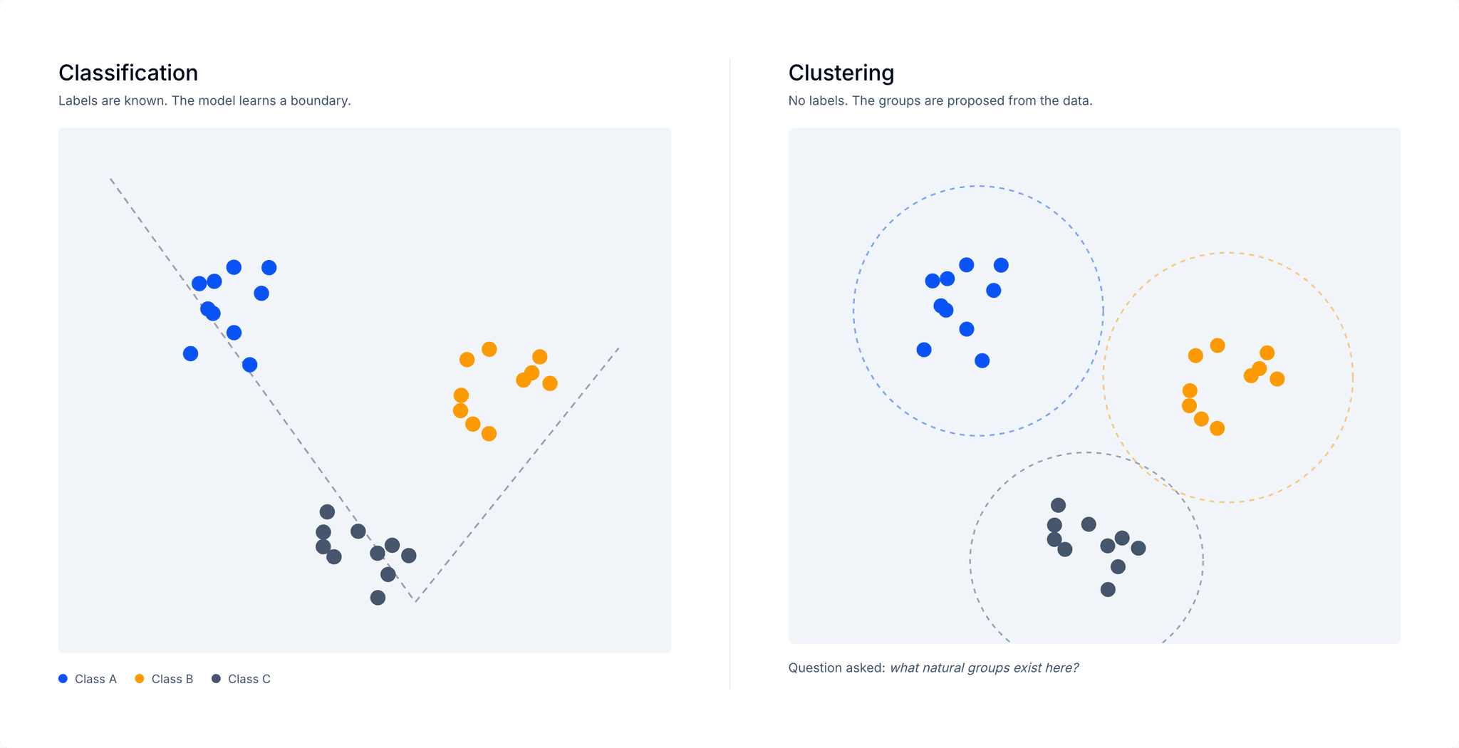
The cleanest way to place clustering is against its supervised sibling. Classification learns a decision boundary from labeled examples: you already know the categories, and the model's job is to sort new points into them. Clustering proposes the categories in the first place, from unlabeled data. Classification answers "which known class is this?" Clustering answers "what natural groups exist here at all?"1
The distinction blurs in practice, and that is where clustering for classification earns its place. When labels are scarce or expensive, a common pattern is to cluster first, inspect and label the resulting groups, then train a classifier on those labels. This cluster-then-label workflow, a form of weak supervision, is how a lot of production annotation actually starts. Clustering for classification also shows up as feature engineering, where cluster assignments become an extra input column for a downstream supervised model.
Use clustering for classification carefully, though. The clusters carry whatever bias your representation and metric introduced, so labels derived from them inherit that bias. Treat the partition as a hypothesis to validate, which is exactly the discipline the rest of this guide is about, before it becomes training data for a classifier.
Clustering runs one way: raw observations, then a representation (features or embeddings), then a distance d(x, y), then the model. The algorithm never sees your data. It sees only the distances, or a similarity matrix derived from them. Two observations are the same kind of thing if and only if the metric says so, which means every downstream property (cluster shapes, what counts as an outlier, which validation indices are even defined) is inherited from a choice you made upstream.
The corollary is the one people resist. A better algorithm cannot repair a bad metric. It will faithfully recover the structure that the wrong notion of similarity created. So the most common failure mode is quietly reshaping the representation until a favorite algorithm produces clean output, which is changing the question to suit the answer you wanted.
Choosing the feature set is choosing the question. Take a set of houses. Price and taxes give you market segments. Floor area and room count give size classes. Latitude and longitude give neighborhoods. Same houses, different clusterings, none of them wrong, because they answer different questions. "Use all the features" feels neutral, but it weights each aspect of the data in proportion to how many columns happen to describe it. Twenty size columns and three style columns means you clustered on size and told yourself you stayed objective.
K-means clustering is the most widely used clustering algorithm, and the right place to start because its assumptions are explicit. It defines a cluster as a set of points near a common center. Lloyd's algorithm runs the loop: assign each point to the nearest center, recompute each center as the mean of its members, and repeat until nothing moves. What it minimizes is the within-cluster sum of squares.
Those mechanics imply hard requirements. K-means clustering needs a vector space where the mean is a meaningful object, comparable feature scales, and roughly isotropic geometry (clusters about the same size and spread). Give it that and it scales to very large datasets and recovers convex, comparably sized blobs well. It fails when clusters are elongated, nested, or unequal in size or density, when the number of clusters k is genuinely unknown, when outliers are present and drag the means, or when all you have is a distance matrix rather than coordinates.
One caution people forget: k-means clustering minimizes within-cluster variance, so it is biased toward producing roughly spherical, roughly equal-sized clusters. If it returns tidy clusters, that tidiness is partly an artifact of what it optimizes, not evidence of real structure. Moreover, every element is assigned to a cluster no matter how bad an outlier it is, so noise never gets to stay noise. In practice you will reach for k-means++ initialization, MiniBatch k-means for very large n, and k-medoids when you only have a distance matrix.2
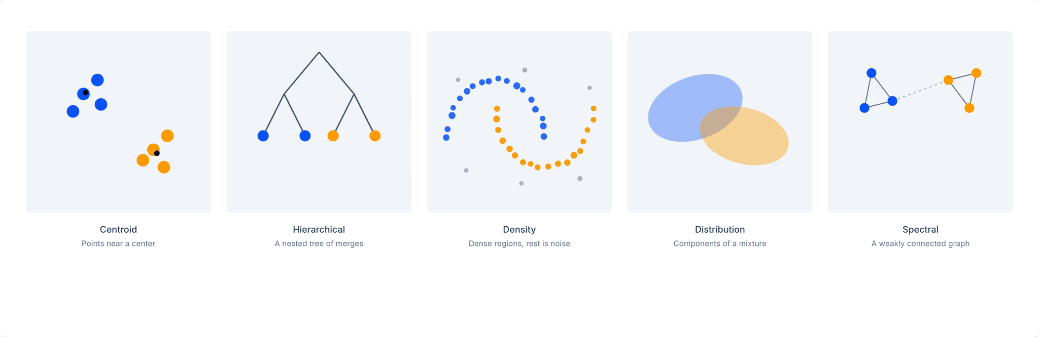
K-means is one family among several, and the five main types of clustering are not interchangeable tools. Each is a different answer to the question "what is a cluster," which makes your choice a claim about how your data was generated.
Centroid-based (k-means, k-medoids): a cluster is a set of points near a common center. Convex blobs, very large scale, needs a vector space.
Hierarchical clustering: a cluster is a level in a nested sequence of merges. The linkage rule (single, complete, average, Ward) matters more than the choice of hierarchical clustering itself; single and Ward on the same data can produce unrecognizable partitions. It works from any distance matrix and lets you pick k after seeing the tree, but it costs O(n²) memory, so it stops scaling around tens of thousands of points.
Density-based (DBSCAN, HDBSCAN, OPTICS): a cluster is a connected region of high density separated by sparse space. Whatever is left over is labeled noise rather than forced into a group. Density needs contrast, and the curse of dimensionality dilutes that contrast as the number of dimensions increases. DBSCAN defines clusters using a single global neighborhood scale, whereas HDBSCAN considers density structure across a range of scales and extracts the most persistent clusters.
Distribution-based (Gaussian mixtures): a cluster is a component of the mixture that generated the data. You get soft assignments, uncertainty, and BIC as a principled way to select k, at the price of assuming a distributional form and elliptical shapes.
Spectral: a cluster is a weakly connected part of a similarity graph. It recovers non-convex and manifold shapes and needs only a similarity matrix, but naive versions cost O(n³) and are sensitive to the affinity scale.
These types of clustering map to different domain claims. Choosing HDBSCAN asserts there are genuinely distinct groups with sparse space between them, and that some points belong to none. That is a falsifiable statement about your data, not a software preference.
An at-a-glance overview of clustering methods makes the trade-offs concrete. There is no best column, only the family that matches your constraints.
| Family | Needs k? | Cluster shape | Noise label | Scales to | Metric flexibility |
|---|---|---|---|---|---|
| Centroid | Yes | Convex, isotropic | No | Very large n | Vector space (medoids: any matrix) |
| Hierarchical | No, cut later | Depends on linkage | No | ~10⁴ (O(n²) memory) | Any distance matrix (except Ward) |
| Density | No | Arbitrary | Yes, explicit | Large, with a spatial index | Any distance matrix |
| Distribution | Yes, or a prior | Elliptical | Via low likelihood | Medium n | Vector space |
| Spectral | Yes | Arbitrary, manifold | No | ~10⁴ naive | Any similarity matrix |
The scikit-learn clustering documentation has a well-known figure that runs 11 algorithms across six toy datasets, and it is worth studying for two rows in particular.3 The bottom row is uniform noise, and most methods still return confident, tidy partitions of nothing; only the density methods say the honest thing and label it noise. But read the row just above it too, the three blobs with two of them partly overlapping: there the density methods are the ones that struggle, merging the touching pair or shaving its edge into noise, while a centroid or distribution method that knows to expect three groups recovers them cleanly. The pair of rows is the whole point. Which family wins is decided by the reality of the problem, not by a ranking, and there is no universally best method.
That is also why the single cheapest check in clustering is the null test: run the same pipeline on structureless data (uniform noise, or a shuffled copy of your own) and look at what it returns. Every method carves noise into confident partitions, so seeing that output is what lets you recognize real structure when you have it. The bottom row of that figure is exactly this test run once, and the rest of this guide turns it into a habit.
The algorithmic differences between families are easiest to feel with real numbers. The two comparisons below are the ones that matter most in practice, and both are reproducible with a fixed random_state.
The clearest way to feel the curse of dimensionality is to run dbscan vs kmeans thinking on a high-dimensional set. We used scikit-learn's load_digits, 1,797 handwritten digits as 64-dimensional pixel vectors, with 10 true classes, and ran the same two clusterers in two regimes: on the raw 64 dimensions, and after reducing to 10 with UMAP. The two methods are k-means (centroid) and HDBSCAN (density), so what follows is an HDBSCAN-vs-k-means comparison. HDBSCAN is the hierarchical successor to DBSCAN: instead of committing to a single global neighborhood radius the way DBSCAN does, it scans a whole range of density levels and keeps the clusters that persist across them, which also makes this a hdbscan vs dbscan check of whether that one fixed radius could have kept up. Density has a textbook case it is built for, arbitrary shapes with clean space between them; digits, as the numbers below show, are the opposite kind of problem.
from sklearn.datasets import load_digits
from sklearn.preprocessing import StandardScaler
from sklearn.cluster import KMeans
from sklearn.metrics import adjusted_rand_score
import umap
import hdbscan

X, y = load_digits(return_X_y=True)
Xs = StandardScaler().fit_transform(X)

def ari_kmeans(data):
km = KMeans(n_clusters=10, n_init=10, random_state=42).fit(data)
return adjusted_rand_score(y, km.labels_)

def ari_hdbscan(data):
hdb = hdbscan.HDBSCAN(min_cluster_size=30).fit(data)
return adjusted_rand_score(y, hdb.labels_)

# Regime 1: raw 64-d pixels
print(ari_kmeans(Xs), ari_hdbscan(Xs))     # 0.534   0.06

# Regime 2: UMAP -> 10-d, then the same two clusterers
emb = umap.UMAP(n_neighbors=30, min_dist=0.0,
n_components=10, random_state=42).fit_transform(Xs)
print(ari_kmeans(emb), ari_hdbscan(emb))   # 0.875   0.797
Adjusted Rand Index (ARI) measures agreement with the true labels, where 0 is random and 1 is perfect. Four runs, one table:
| Representation | k-means (ARI) | HDBSCAN (ARI) |
|---|---|---|
| Raw 64-d pixels | 0.534 | 0.06 |
| UMAP → 10-d | 0.875 | 0.797 |
Read down the columns first, because that is the curse of dimensionality in a single number. Reducing the space lifts both methods, and it rescues HDBSCAN completely: 0.06 to 0.797, from barely-above-random to a real partition. In 64 dimensions the density contrast has collapsed, so HDBSCAN has almost nothing to cut on and dumps most points into noise; k-means still carves the space into convex cells and limps to 0.534. UMAP restores contrast by compressing the data into a low-dimensional space where the real gaps reopen, and the density method comes alive. This is the practical answer to hdbscan vs dbscan: HDBSCAN's variable-density extraction is what survives the reduction, where a single global radius would not.
Now read across the rows, because they carry the less comfortable lesson. In both regimes k-means edges out HDBSCAN (0.534 vs 0.06, then 0.875 vs 0.797). Density is not universally better, and this example is not the one where it wins. Handwritten-digit classes overlap heavily, and where clusters bleed into one another a centroid method that assigns every point can beat a density method that recovers only the dense cores and calls the ambiguous middle noise. A caveat on that word overlap: some of it is real in the space where the clustering happens, but any 2D picture of this data exaggerates it, because a scatter of 64-dimensional digits is a projection, and two points from different classes can land on top of each other simply because the features that separate them are not among the two axes drawn. Trust the ARI computed in the space you clustered over what a scatter appears to show. Which family wins is decided by the shape of the problem, overlap here, not by a ranking, exactly the point the next comparison makes from the other side.
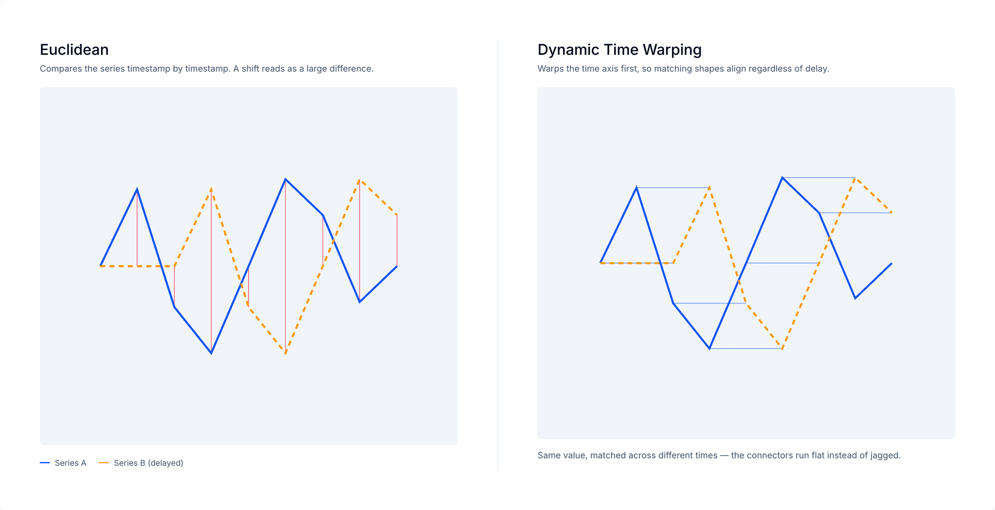
Time series make the metric decision impossible to ignore. Two recordings can trace the same shape at different speeds or with a slight delay, and any sensible person would call them the same type. Euclidean distance disagrees, because it compares the series timestamp by timestamp, so a small shift reads as a large difference.
We used the UCR Trace dataset, 200 transient signals of length 275 across four classes, signals that share shapes but start at different times. The comparison is k-means with Euclidean distance against k-means with Dynamic Time Warping (DTW), which warps the time axis to align comparable shapes before measuring distance.
from tslearn.datasets import UCR_UEA_datasets
from tslearn.clustering import TimeSeriesKMeans
from tslearn.preprocessing import TimeSeriesScalerMeanVariance
from sklearn.metrics import adjusted_rand_score

X_tr, y_tr, X_te, y_te = UCR_UEA_datasets().load_dataset("Trace")
X = TimeSeriesScalerMeanVariance().fit_transform(list(X_tr) + list(X_te))
y = list(y_tr) + list(y_te)

eucl = TimeSeriesKMeans(n_clusters=4, metric="euclidean", random_state=42).fit(X)
print(adjusted_rand_score(y, eucl.labels_))        # 0.328

dtw = TimeSeriesKMeans(n_clusters=4, metric="dtw", random_state=42).fit(X)
print(adjusted_rand_score(y, dtw.labels_))         # 0.664
Euclidean k-means scores ARI 0.328. Switching only the metric to DTW lifts it to 0.664, roughly doubling agreement with the true classes on identical data and the same algorithm. The metric decided the problem.
DTW is not a free upgrade. On the ECG5000 dataset, whose heartbeats are already aligned to the R-peak, DTW actually underperformed Euclidean in our run (0.408 down to 0.326), because there was no misalignment left to correct and warping only introduced spurious matches. DTW is also quadratic in sequence length and not a proper metric, since it can violate the triangle inequality.4 Use it when your signals share shape but drift in time.
There is a sharper move hiding here, and it is worth the extra step. Switching to DTW fixed the metric, but we kept feeding that metric to k-means, which still assumes the clusters are round and equally sized. We can check that assumption directly. Classical multidimensional scaling (MDS) tries to embed a distance matrix into a Euclidean space and reports, through its eigenvalue spectrum, how many dimensions that actually takes and whether the geometry is isotropic. Run it on the Trace DTW matrix and the answer is emphatic: one axis carries about 91 percent of the positive eigenvalue mass, the effective dimensionality is barely above one, and a slice of the mass is even negative, which means DTW does not embed cleanly into a Euclidean space at all. The clusters are long and thin, not round, so k-means is the wrong shape of tool no matter how good the metric is.
import numpy as np
import hdbscan
from tslearn.metrics import cdist_dtw

# DTW distance matrix on the same scaled Trace series
D = cdist_dtw(X, n_jobs=-1).astype(np.float64)

# Classical MDS: does DTW embed into an isotropic Euclidean space?
n = D.shape[0]
J = np.eye(n) - np.ones((n, n)) / n
B = -0.5 * J @ (D ** 2) @ J
w = np.sort(np.linalg.eigvalsh((B + B.T) / 2))[::-1]
pos = w[w > 0]
print(pos[0] / pos.sum())                 # 0.907  -> one axis holds ~91% of the mass
print(pos.sum() ** 2 / (pos ** 2).sum())  # 1.21   -> ~1 effective dimension

# HDBSCAN straight on the DTW matrix, no vector space assumed
h = hdbscan.HDBSCAN(min_cluster_size=10, min_samples=1,
metric="precomputed").fit(D)
print(adjusted_rand_score(y, h.labels_)) # 1.000The plot above shows only the top two principal coordinates of the MDS representation, so part of the information in the DTW matrix never reaches the page. That is why classes 3 and 4 look fully overlapped along the left arm: what separates them lives in a direction the two axes leave out. HDBSCAN never sees this projection; it works from the full distance matrix, which is how it tells those two classes apart cleanly even though they appear on top of each other here.
The fix follows from the diagnosis. HDBSCAN consumes the DTW distance matrix directly and never assumes a vector space or a cluster shape, so it is free of the assumption MDS just showed to be violated. Fed the same distances, it recovers the four classes perfectly, ARI 1.000, across a wide range of min_cluster_size. Right metric, then a model whose assumptions the metric actually satisfies, checked rather than hoped for.
Beyond picking a family, a handful of clustering techniques decide whether any of them will work. These are the craft of step one, and time spent here is almost never wasted.
Scaling and normalization set the implicit weights. Unscaled features are weighted by their measurement units, so standardize roughly symmetric features, use robust (median and IQR) scaling when heavy tails or artifacts are present, and normalize within a subject or time series before pooling when baselines differ across individuals and you do not want those baselines to dominate.
Feature engineering makes the aspect you care about visible to the metric. Ratios and proportions buy scale-invariance (price per square meter, term frequencies). Differences from a baseline do the same job by subtraction. Rolling windows and summaries collapse variable-length objects into fixed-length descriptors so they can be compared at all.
Dimensionality reduction is often mandatory rather than optional. As dimension grows, the nearest and farthest points become nearly equidistant, so the idea of a neighborhood dissolves. This is the curse of dimensionality, and it flattens density estimates and strips Euclidean distance of discriminative power.5 Reduce with PCA as a cheap first move, or UMAP before a density method, and treat the UMAP into HDBSCAN pattern as a standard technique for high-dimensional data. Handle that pattern with care, though: a nonlinear reduction like UMAP is expressive enough to invent gaps that were not in the data, so it can manufacture clusters as readily as it reveals them. Run the null test through the whole reduce-then-cluster pipeline before you trust its output.
Choosing a metric comes down to which invariances your domain requires. Should doubling a feature change nothing? Use ratios or cosine. Is only the ordering trustworthy? Use rank-based distances. Do two trajectories with the same shape at different tempos belong together? Use a warping metric like DTW, and accept that you lose the vector space in exchange.
A partition passes review only if it answers four questions honestly. For each, the failing case looks plausible; only a number computed against a baseline separates it from a real finding.
Are they real? Run k-means on 420 uniformly random points and it returns tidy clusters with a silhouette score around 0.41, the kind of value that gets reported as moderate structure. It is a tessellation of noise. So the question to test is not "are there clusters" but "is this structure stronger than what my pipeline produces on structureless data with the same marginals?"
Are they stable? Real clusters survive being disturbed. Resample the data with the bootstrap, or add a little noise to it, and refit the entire pipeline (scaling, reduction, and clustering, not just the last step): structure that is genuinely there should survive small perturbations. Match each new cluster to its original by overlap, and score the agreement with the Jaccard index. Report it per cluster, never as one global average, because a five-cluster solution typically has two clusters you would defend and three that dissolve. One caveat when resampling: a small cluster can dissolve simply because it holds few elements and rarely gets sampled intact, not because it lacks structure, so read low stability on a tiny cluster alongside its size rather than as a verdict on its own.
Are they distinct, and in what way? Position and spread are separate claims. PERMANOVA tests whether groups differ in location directly on a distance matrix, which matters when you have no coordinates.6 PERMDISP tests whether their spread differs. Run both, because a location test alone would miss two groups that share a center but differ sharply in variance. To see which features actually separate the groups, a per-feature Kruskal-Wallis test asks whether a feature's values differ across clusters, and its effect size (epsilon-squared) is readable as the share of that feature's variance explained by cluster membership rather than by variation within clusters, which is what tells you a split is driven by something real and not by one noisy column. For density-based partitions, lean on density-aware validity indices such as DBCV rather than convexity-biased ones. At the sample sizes production data reaches, a p-value is close to automatic, so report effect sizes with intervals (Cliff's delta, epsilon-squared) as the statistic that carries information.
Are they useful? Tie the partition back to the reason you built it. A clustering that is excellent for compression can be worthless for taxonomy, and only the downstream use tells you which numbers mattered.
There is a circularity trap underneath all of this. If you form groups by maximizing separation on features X and then test whether the groups differ on X, the test rejects because you built the groups to make it reject. Under the null of a single homogeneous population, standard tests after clustering reject at rates approaching certainty.7 The fixes, in order of practicality: hold out variables the clustering never saw and test on those, split the sample, use selective inference designed for clustering,7 or report effect sizes and drop the inferential claim.
If you take one habit from this guide, take the null-model test. Run the whole pipeline, scaling and reduction and clustering and indices, on a column-permuted copy of your data, one where each feature is shuffled independently so every marginal is preserved and all joint structure is destroyed. If that copy scores about as well as your real data, the pipeline manufactures clusters and nothing downstream is evidence. Our predictive modeling work leans on exactly this discipline before any partition reaches a stakeholder.
A few habits show up again and again, and each one silently corrupts a result.
Reading inter-cluster distances, cluster sizes, or density off a t-SNE or UMAP plot. These embeddings separate clusters but do not preserve geometry; the gaps between islands are set by the optimizer, not the data, so a claim that "these two clusters are closer" has no support. The reverse trap is just as common: points from different clusters can pile on top of each other in the plot because the features that separate them are not among the two axes shown, so overlap you see on the page need not be overlap that exists in the data. Validate in the space you clustered in and use the projection only to communicate.
Resampling at the wrong unit. If the independence sits at the instance level, bootstrapping highly correlated sub-instances or rows can give stability numbers so high they are meaningless. Resample at the level where observations are actually independent.
Tuning parameters against an index that doesn't fit your method. Silhouette rewards convex, compact clusters, so optimizing a density-based result against it just penalizes the shapes you chose density to find. Use DBCV,8 the density-aware validity index, for density-based partitions.
Never running the pipeline on a null dataset. This is the same point as the column-permutation test, and it is the cheapest insurance in the entire workflow. It is hard to claim there is structure without first knowing what true randomness looks like coming out of your own pipeline, so make that null run the reference you judge every real result against.
You rarely need to try every family. What you already know about the problem eliminates most of them.
If you know k, have very large n, and expect convex blobs, start with k-means clustering or MiniBatch k-means. If k is unknown, you expect genuine outliers, and shapes may be arbitrary, use HDBSCAN, after reducing dimension if the data is high-dimensional. If all you have is a distance matrix, your options are k-medoids, average-linkage hierarchical clustering, or HDBSCAN on the precomputed distances. If n runs into the millions, avoid anything with O(n²) memory, which rules out standard hierarchical and spectral methods. If the data is very high-dimensional, reduce first and treat that as mandatory.9
One cross-check is worth more than any single index. If a density method and a hierarchical method on the same representation broadly agree, that agreement is strong evidence, because the two definitions of cluster are different and they converged anyway.
Clustering algorithms reward teams who spend their effort in the right place. Three steps, in order: choose the representation and the metric, which is where the problem is actually defined and where most projects fail; pick the model whose definition of "cluster" matches the space you built; then validate. Four questions before you call it a result: are the groups real, stable, distinct, and useful, answered in the space you clustered in and against a null run through the same pipeline.
This is how we run unsupervised work in production at Pento, no client names and no proprietary data required: representation and metric first, a model chosen to match, and no partition treated as a result until it survives a null run through the same pipeline.
If you are weighing an unsupervised project and want to pressure-test the representation, the metric, or the validation plan before committing engineering time, book a call and we will compare notes.
Classification vs Clustering in Machine Learning (DataCamp) ↩
Dynamic Time Warping (Müller, Information Retrieval for Music and Motion) ↩
When Is "Nearest Neighbor" Meaningful? (Beyer et al., 1999) ↩
A new method for non-parametric multivariate analysis of variance (Anderson, 2001) ↩
Selective inference for hierarchical clustering (Gao, Bien & Witten, 2022) ↩ ↩2
Density-Based Clustering Validation (Moulavi et al., 2014) ↩
CONTACT US
Work with Pento to turn promising AI experiments into systems that perform reliably in production, with the right architecture, delivery model, and engineering support.